SSC/Stability/BiPolytropes/RedGiantToPN: Difference between revisions
| (48 intermediate revisions by 2 users not shown) | |||
| Line 19: | Line 19: | ||
==Preface== | ==Preface== | ||
Go [[SSC/Structure/Polytropes/VirialSummary#StahlerSchematic|here]] for Stahler schematic. | |||
<table border="0" align="left" cellpadding="10"><tr><td align="center"> | |||
<table border="1" align="left" cellpadding="2"> | |||
<tr><td align="center"> | |||
[[File:Stahler1983TitlePage0.png|center|100px|ApJ reference]] | |||
</td></tr> | |||
<tr><td align="center"> | |||
[[File:Stahler MRdiagram1.png|left|100px|Stahler Schematic]] | |||
</td></tr> | |||
</table> | |||
</td></tr></table> | |||
<table border="0" cellpadding="8" align="right"> | <table border="0" cellpadding="8" align="right"> | ||
| Line 31: | Line 44: | ||
</tr> | </tr> | ||
</table> | </table> | ||
As has been detailed in an [[SSC/Stability/BiPolytropes#Overview|accompanying chapter]], we have [[SSC/Stability/InstabilityOnsetOverview#Marginally_Unstable_Pressure-Truncated_Gas_Clouds|successfully analyzed the relative stability of pressure-truncated polytopes]]. The curves shown here on the right in Figure 1 graphically present the mass-radius relationship for pressure-truncated model sequences having a variety of polytropic indexes, as labeled, over the range <math>1 \le n \le 6</math>. ([[SSC/Stability/InstabilityOnsetOverview#Turning_Points_along_Sequences_of_Pressure-Truncated_Polytropes|Another version of this figure]] includes the isothermal sequence.) | As has been detailed in an [[SSC/Stability/BiPolytropes#Overview|accompanying chapter]], we have [[SSC/Stability/InstabilityOnsetOverview#Marginally_Unstable_Pressure-Truncated_Gas_Clouds|successfully analyzed the relative stability of pressure-truncated polytopes]]. The curves shown here on the right in Figure 1 graphically present the mass-radius relationship for pressure-truncated model sequences having a variety of polytropic indexes, as labeled, over the range <math>1 \le n \le 6</math>. ([[SSC/Stability/InstabilityOnsetOverview#Turning_Points_along_Sequences_of_Pressure-Truncated_Polytropes|Another version of this figure]] includes the isothermal sequence, for which <math>n = \infty</math>.) | ||
<br /> | |||
Along each sequence for which <math>n \ge 3</math>, the green filled circle identifies the model with the largest mass. This maximum-mass model is the polytropic analogue of the Bonnor-Ebert mass, which was identified independently by {{ Ebert55 }} and {{ Bonnor56 }} in the context of studies of pressure-truncated ''isothermal'' equilibrium configurations. | |||
<ol type="1"> | |||
<li>The maximum-mass model's position along each sequence has been determined analytically by setting <math>\partial M_\mathrm{tot}/\partial \xi \biggr|_\tilde{\xi} = 0.</math></li> | |||
<li> | |||
By solving the LAWE associated with various models along each equilibrium sequence, we have shown that the eigenfrequency of the fundamental-mode of radial oscillation is zero for each one of these maximum-mass models. | |||
<ol type="a"> | |||
<li>Solutions to the LAWE were initially obtained via numerical integration techniques, in which case we were only able to make this association approximately;</li> | |||
<li>To our surprise, we also have been able to determine ''analytically'' an expression that defines the eigenfunction of the marginally unstable equilibrium model along each sequence <math>(n \ge 3)</math>; as a result we have been able to show that the eigenfrequency associated with the maximum-mass model is ''precisely'' zero.</li> | |||
</ol> | |||
As a consequence, we know that each green circular marker identifies the point along its associated sequence that separates dynamically stable (larger radii) from dynamically unstable (smaller radii) models.</li> | |||
</ol> | |||
<font color="red">'''Key Realization:'''</font> ''Along sequences of pressure-truncated polytropes, the maximum-mass models identify precisely where the onset of dynamical instability occurs.'' | <font color="red">'''Key Realization:'''</font> ''Along sequences of pressure-truncated polytropes, the maximum-mass models identify precisely where the onset of dynamical instability occurs.'' | ||
| Line 37: | Line 63: | ||
---- | ---- | ||
<table border="0" cellpadding="8" align="right"> | |||
<tr> | |||
<th align="center"><font size="-1">'''Figure 2: Equilibrium Sequences of Bipolytropes'''</font> <br /><p> | |||
<font size="-1">'''with <math>(n_c,n_e) = (5,1)</math> and Various <math>\mu_e/\mu_c</math>'''</font> | |||
</th> | |||
</tr> | |||
<tr> | |||
<td align="center" colspan="1"> | |||
[[File:TurningPoints51Bipolytropes.png|300px|Extrema along Various Equilibrium Sequences]] | |||
</td> | |||
</tr> | |||
</table> | |||
Using similar techniques, we have successfully analyzed the relative stability of bipolytropic configurations that have <math>(n_c, n_e) = (5, 1)</math>. Our analytically constructed equilibrium model sequences replicate the ones originally presented by {{ EFC98 }} for this same pair of bipolytropic indexes; and they serve as analogues of the sequences that were constructed numerically by {{ HC41 }} and {{ SC42 }} for bipolytropic configurations that have <math>(n_c, n_e) = (\infty, \tfrac{3}{2})</math>. | |||
Following {{ HC41hereafter }} and {{ SC42hereafter }}, we have found it particularly useful to label each equilibrium model according to the key structural parameters, <math>q \equiv r_\mathrm{core}/R_\mathrm{surf}</math> and <math>\nu \equiv M_\mathrm{core}/M_\mathrm{tot}</math>. The curves shown here on the right in Figure 2 graphically present the <math>q - \nu</math> relationship for bipolytropic model sequences that have a variety of molecular-weight jumps, <math>\tfrac{1}{4} \le \mu_e/\mu_c \le 1</math>, at the core-envelope interface, as labeled. Along each Fig. 2 sequence for which <math>\mu_e/\mu_c \le \tfrac{1}{3}</math>, the green filled circle identifies the model with the largest mass ratio, <math>\nu</math>. This maximum-mass model is a polytropic analogue of the Schönberg-Chandrasekhar mass limit, which was identified by {{ HC41hereafter }} and {{ SC42hereafter }} in the context of their studies of stars with isothermal cores. | |||
<ol type="1"> | |||
<li>The maximum-mass model's position along each sequence has been determined analytically by setting <math>\partial \nu/\partial q = 0.</math></li> | |||
<li> | |||
By solving the LAWE associated with various models along each equilibrium sequence, we have shown that the eigenfrequency of the fundamental-mode of radial oscillation is zero for each one of these maximum-mass models. | |||
<ol type="a"> | |||
<li>Solutions to the LAWE were initially obtained via numerical integration techniques, in which case we were only able to make this association approximately;</li> | |||
<li>To our surprise, we also have been able to determine ''analytically'' an expression that defines the eigenfunction of the marginally unstable equilibrium model along each sequence <math>(n \ge 3)</math>; as a result we have been able to show that the eigenfrequency associated with the maximum-mass model is ''precisely'' zero.</li> | |||
</ol> | |||
As a consequence, we know that each green circular marker identifies the point along its associated sequence that separates dynamically stable (larger radii) from dynamically unstable (smaller radii) models.</li> | |||
</ol> | |||
indexes, as labeled, over the range <math>1 \le n \le 6</math>. | |||
<!-- | |||
<font color="red">'''The principal question is:'''</font> ''Along bipolytropic sequences, are maximum-mass models (identified by the solid green circular markers in Fig. 2) associated with the onset of dynamical instabilities?''</span> For more details, look [[SSC/Stability/BiPolytropes/51Models#Structure|here]]. | <font color="red">'''The principal question is:'''</font> ''Along bipolytropic sequences, are maximum-mass models (identified by the solid green circular markers in Fig. 2) associated with the onset of dynamical instabilities?''</span> For more details, look [[SSC/Stability/BiPolytropes/51Models#Structure|here]]. | ||
--> | |||
<table border="1" align="center" cellpadding="3"> | <table border="1" align="center" cellpadding="3"> | ||
| Line 852: | Line 910: | ||
</table> | </table> | ||
====Sequence Plots==== | ====Fixed Interface Pressure Sequence Plots==== | ||
A plot of <math>M_\mathrm{tot}~\biggl[K_c^{5}K_e G^{-6}\biggr]^{-1 / 4}</math> versus <math>R~\biggl[K_e G^{-1} \biggr]^{-1/2}</math> at <font color="red"><b>fixed interface pressure</b></font> will be generated via the relations, | A plot of <math>M_\mathrm{tot}~\biggl[K_c^{5}K_e G^{-6}\biggr]^{-1 / 4}</math> versus <math>R~\biggl[K_e G^{-1} \biggr]^{-1/2}</math> at <font color="red"><b>fixed interface pressure</b></font> will be generated via the relations, | ||
<table align="center" cellpadding="8"> | <table align="center" cellpadding="8"> | ||
| Line 1,435: | Line 1,493: | ||
</table> | </table> | ||
For <math>\mu_e/\mu_c = 1.00</math> the <font color="red">solution to this expression is <math>\xi_i = 1.668462981</math></font>. | For <math>\mu_e/\mu_c = 1.00</math> the <font color="red">solution to this expression is <math>\xi_i = 1.668462981</math></font>. | ||
</td></tr></table> | </td></tr></table> | ||
| Line 1,523: | Line 1,582: | ||
<table border="1" cellpadding="3" align="center"> | <table border="1" cellpadding="3" align="center"> | ||
<tr> | <tr> | ||
< | <td align="center" colspan="3"> | ||
Equilibrium Sequences of <math>(n_c, n_e) = (5, 1)</math> BiPolytropes Having <math>\mu_e/\mu_c = 1.0</math> | Equilibrium Sequences of <math>(n_c, n_e) = (5, 1)</math> BiPolytropes Having <math>\mu_e/\mu_c = 1.0</math><br /> | ||
</ | (viewed from several different astrophysical perspectives) | ||
</td> | |||
</tr> | </tr> | ||
<tr> | <tr> | ||
<td align="center" colspan="1">(Interface Pressure<math>)^{1 / 3}</math> vs. Radius<br />(Fixed Total Mass)</td> | |||
<td align="center" colspan="1">Mass vs. Radius<br />(Fixed Interface Pressure)</td> | <td align="center" colspan="1">Mass vs. Radius<br />(Fixed Interface Pressure)</td> | ||
<td align="center" colspan="1">Mass vs. Central Density<br />(Fixed Interface Pressure)</td> | <td align="center" colspan="1">Mass vs. Central Density<br />(Fixed Interface Pressure)</td> | ||
</tr> | </tr> | ||
<tr> <td align="center" colspan="1"> | <tr> | ||
<td align="center" colspan="1"> | |||
[[File:MuRatio100PressureVsVolumeA.png|350px|center|Pressure vs Volume]] | |||
</td> | |||
<td align="center" colspan="1"> | |||
[[File:MuRatio100MassVsRadiusA.png|350px|Total Mass vs Radius]] | [[File:MuRatio100MassVsRadiusA.png|350px|Total Mass vs Radius]] | ||
</td> | </td> | ||
| Line 1,538: | Line 1,603: | ||
</td> | </td> | ||
</tr> | </tr> | ||
<table border="0" align="center" cellpadding="8"><tr><td align="left"> | <tr> | ||
<td align="center"> | |||
<math>\biggl(\frac{\mu_e}{\mu_c}\biggr)^{-4} \biggl(\frac{2}{\pi}\biggr) A^2\eta_s^2</math> | |||
<br />vs.<br /> | |||
<math>\biggl(\frac{\mu_e}{\mu_c}\biggr)^3 \biggl(\frac{\pi}{2^3}\biggr)^{1 / 2} \frac{1}{A^2\eta_s}</math> | |||
</td> | |||
<td align="center"> | |||
<math>\biggl(\frac{\mu_e}{\mu_c}\biggr)^{-3/2} \biggl(\frac{2}{\pi}\biggr)^{1 / 2} A\eta_s</math> | |||
<br />vs.<br /> | |||
<math>\frac{\eta_s}{\sqrt{2\pi}}</math> | |||
</td> | |||
<td align="center"> | |||
<math>\biggl(\frac{\mu_e}{\mu_c}\biggr)^{-3/2} \biggl(\frac{2}{\pi}\biggr)^{1 / 2} A\eta_s</math> | |||
<br />vs.<br /> | |||
<math>\log_\mathrm{10}\biggl[\biggl(\frac{\mu_e}{\mu_c}\biggr)^{-5/2}\theta_i^{-5} \biggr]</math> | |||
</td> | |||
</tr> | |||
<tr> | |||
<td align="left" colspan="3">NOTE: In all three diagrams, the dashed vertical line identifies the value of the abscissa when it is evaluated for the interface location, <math>\xi_i = 1.668462981</math>. In each case, this vertical line intersects a key turning point along the model sequence. | |||
</td> | |||
</tr> | |||
</table> | |||
<table border="0" align="center" cellpadding="8"><tr><td align="left"> | |||
[[File:DataFileButton02.png|right|60px|file = Dropbox/WorkFolder/Wiki edits/BiPolytrope/TwoFirstOrderODEs/Bipolytrope51New.xlsx --- worksheet = MuRatio100Fund]]Data values drawn from worksheet "MuRatio100Fund" … | [[File:DataFileButton02.png|right|60px|file = Dropbox/WorkFolder/Wiki edits/BiPolytrope/TwoFirstOrderODEs/Bipolytrope51New.xlsx --- worksheet = MuRatio100Fund]]Data values drawn from worksheet "MuRatio100Fund" … | ||
| Line 1,570: | Line 1,658: | ||
</td></tr></table> | </td></tr></table> | ||
=== | ====Temporary Excel Interpolations==== | ||
<font color="red">HERE</font> | |||
=== | <table border="1" align="center" cellpadding="5"> | ||
<tr> | |||
<td align="center" colspan="6"><b>Properties of Turning-Points Along Sequences Having Various <math>\mu_e/\mu_c</math></b></td> | |||
< | </tr> | ||
<tr> | <tr> | ||
<td align=" | <td align="center" rowspan="2"><math>\frac{\mu_e}{\mu_c}</math></td> | ||
<math> | <td align="center" rowspan="2"><math>\xi_i</math></td> | ||
<td align="center"><math>P_i</math></td> | |||
</math> | <td align="center"><math>R</math></td> | ||
</td> | <td align="center"><math>M_\mathrm{tot}</math></td> | ||
<td align="center"> | <td align="center"><math>\log_{10}(\rho_\mathrm{max})</math></td> | ||
<math> | |||
</td> | |||
<td align=" | |||
<math> | |||
= | |||
\ | |||
</math> | |||
</tr> | </tr> | ||
<tr> | |||
<td align="center" colspan="2">(Fixed <math>M_\mathrm{tot}</math>)</td> | |||
<td align="center" colspan="2">(Fixed <math>P_i</math>)</td> | |||
</tr> | |||
<tr> | |||
<td align="right">1.000</td> | |||
<td align="right">1.6684629814</td> | |||
<td align="right">12.03999149</td> | |||
<td align="right">0.092175036</td> | |||
<td align="right">3.46986909</td> | |||
<td align="right">0.712724159</td> | |||
</tr> | |||
<tr> | |||
<td align="right">0.9</td> | |||
<td align="right">1.4459132276</td> | |||
<td align="right">13.67957562</td> | |||
<td align="right">0.091291571</td> | |||
<td align="right">3.50879154</td> | |||
<td align="right">0.688526899</td> | |||
</tr> | |||
<tr> | |||
<td align="right">0.8</td> | |||
<td align="right">1.0482530437</td> | |||
<td align="right">17.09391244</td> | |||
<td align="right">0.086279818</td> | |||
<td align="right">3.69798999</td> | |||
<td align="right">0.58112284</td> | |||
</tr> | |||
<tr> | |||
<td align="right">0.75</td> | |||
<td align="right">0.7170001608</td> | |||
<td align="right">20.48027265</td> | |||
<td align="right">0.079651055</td> | |||
<td align="right">3.91920968</td> | |||
<td align="right">0.484075667</td> | |||
</tr> | |||
<tr> | |||
<td align="right">0.74</td> | |||
<td align="right">0.6365283705</td> | |||
<td align="right">21.40307774</td> | |||
<td align="right">0.0777495</td> | |||
<td align="right">3.97973335</td> | |||
<td align="right">0.464464039</td> | |||
</tr> | |||
</table> | |||
===Fixed Total Mass=== | |||
====Equilibrium Sequence Expressions==== | |||
Again, drawing from [[SSC/Structure/BiPolytropes/Analytic51/Pt2#Normalization|previous Examples]] in which <math>\rho_0</math> — as well as <math>K_c</math> and <math>G</math> — is held fixed, equilibrium models obey the relations, | |||
<table border="0" align="center" cellpadding="5"> | |||
<tr> | <tr> | ||
<td align="right"> | <td align="right"> | ||
<math> | <math> | ||
M_\mathrm{tot} | |||
</math> | </math> | ||
</td> | </td> | ||
| Line 1,609: | Line 1,746: | ||
<td align="left"> | <td align="left"> | ||
<math> | <math> | ||
M^*_\mathrm{tot} \biggl[ K_c^{3/2} G^{-3/2} \rho_0^{-1/5} \biggr] | |||
= | = | ||
\biggl[ K_c^{1/2} G^{-1/2} \rho_0^{-2/5} \biggr] \biggl(\frac{\mu_e}{\mu_c}\biggr)^{-1} \frac{\eta_s}{\sqrt{2\pi}~\theta_i^2} | \biggl[ K_c^{3/2} G^{-3/2} \rho_0^{-1/5} \biggr] | ||
\biggl(\frac{\mu_e}{\mu_c}\biggr)^{-2} \biggl(\frac{2}{\pi}\biggr)^{1 / 2} \frac{A\eta_s}{\theta_i} | |||
\, ; | |||
</math> | |||
</td> | |||
</tr> | |||
<tr> | |||
<td align="right"> | |||
<math> | |||
R | |||
</math> | |||
</td> | |||
<td align="center"> | |||
<math>=</math> | |||
</td> | |||
<td align="left"> | |||
<math> | |||
R^* \biggl[ K_c^{1/2} G^{-1/2} \rho_0^{-2/5} \biggr] | |||
= | |||
\biggl[ K_c^{1/2} G^{-1/2} \rho_0^{-2/5} \biggr] \biggl(\frac{\mu_e}{\mu_c}\biggr)^{-1} \frac{\eta_s}{\sqrt{2\pi}~\theta_i^2} | |||
\, ; | \, ; | ||
</math> | </math> | ||
| Line 1,842: | Line 1,999: | ||
====Sequence Plots==== | ====Sequence Plots==== | ||
A plot of <math>P_i\biggl[ K_c^{-10} G^{9} M_\mathrm{tot}^{6} \biggr]</math> versus <math>R^3\biggl[ K_c^{5/2} G^{-5/2} M_\mathrm{tot}^{-2} \biggr]^{3}</math> at fixed | A plot of <math>P_i\biggl[ K_c^{-10} G^{9} M_\mathrm{tot}^{6} \biggr]</math> versus <math>R^3\biggl[ K_c^{5/2} G^{-5/2} M_\mathrm{tot}^{-2} \biggr]^{3}</math> at fixed total mass will be generated via the relations, | ||
<table align="center" cellpadding="8"> | <table align="center" cellpadding="8"> | ||
<tr> | <tr> | ||
| Line 2,451: | Line 2,608: | ||
=Relevant Instabilities= | =Relevant Instabilities= | ||
==Abstract== | |||
The analysis presented by {{ EFC98 }} is essentially an analysis of the <math>q - v</math> diagram. We can determine analytically at what value of <math>\xi_i</math> the core-to-total mass ratio reaches a maximum (<math>\nu_\mathrm{max}</math>) for various values of <math>\mu_e/\mu_c \le 1/3</math>. For example, <math>(\mu_e/\mu_c, \xi_i, \nu_\mathrm{max}) = (\tfrac{1}{4}, 4.9379256, 0.139270157)</math>. Our LAWE analysis shows that '''none''' of these turning points is associated with the onset of a dynamical instability. | |||
On the other hand, our LAWE analysis '''does''' identify a marginally unstable equilibrium configuration along every sequence; even sequences with <math>\tfrac{1}{3} \le \mu_e/\mu_c \le 1</math>. [[SSC/Stability/BiPolytropes/Pt3#Eigenvectors_for_Marginally_Unstable_Models_with_(γc,_γe)_=_(6/5,_2)|For example]], <math>(\mu_e/\mu_c, \xi_i, \nu) = (1, 1.6686460157, 0.497747626)</math>. | |||
==Truncated n = 5 Polytrope== | ==Truncated n = 5 Polytrope== | ||
| Line 2,514: | Line 2,677: | ||
<ul> | <ul> | ||
<li> | <li> | ||
<font color="red">KEY RESULT:</font> | <font color="red">KEY RESULT:</font> | ||
</li> | <ul> | ||
<li>The maximum "Bonnor-Ebert type" mass and external pressure occurs along the sequence precisely at <math>\tilde\xi = 3</math>.</li> | |||
<li>It is precisely at this turning point that the equilibrium model is marginally (dynamically) unstable; the eigenfunction is parabolic.</li> | |||
<li>[[SSC/Stability/InstabilityOnsetOverview#Marginally_Unstable_Pressure-Truncated_Gas_Clouds|For all <math>3 < n < \infty</math>]], the location along the relevant sequence presents an analogous turning point whose location and whose eigenfunction is known analytically.</li> | |||
</ul> | </ul> | ||
==Bipolytropes with (n<sub>c</sub>, n<sub>e</sub>) = (5, 1)== | ==Bipolytropes with (n<sub>c</sub>, n<sub>e</sub>) = (5, 1)== | ||
===q - ν Sequence Plots=== | |||
In [[SSC/Structure/BiPolytropes/Analytic51/Pt2#Model_Sequences|Figure 1 of an accompanying discussion]], we show — via a plot in the <math>(q, \nu)</math> diagram — how the <math>(n_c, n_e) = (5, 1)</math> bipolytrope sequence behaves for various values of the molecular-weight ratio over the range, <math>\tfrac{1}{4} \le (\mu_e/\mu_c) \le 1</math>. | In [[SSC/Structure/BiPolytropes/Analytic51/Pt2#Model_Sequences|Figure 1 of an accompanying discussion]], we show — via a plot in the <math>(q, \nu)</math> diagram — how the <math>(n_c, n_e) = (5, 1)</math> bipolytrope sequence behaves for various values of the molecular-weight ratio over the range, <math>\tfrac{1}{4} \le (\mu_e/\mu_c) \le 1</math>. | ||
| Line 2,559: | Line 2,727: | ||
</div> | </div> | ||
<font color="red">KEY RESULT:</font> Over the range, <math>\tfrac{1}{4} \le (\mu_e/\mu_c) \le \tfrac{1}{3}</math>, there is a value of <math>\nu</math> above which no equilibrium configurations exist. We have determined the location of this "turning point" by setting, <math>d\nu/d\xi = 0</math>; our [[SSC/Structure/BiPolytropes/Analytic51/Pt3#Derivation|derived result]] is, | |||
< | <div align="center"> | ||
< | <table border="0" cellpadding="5"> | ||
< | <tr> | ||
<td align="right"> | |||
<math> | |||
\underbrace{\biggl(\frac{\pi}{2} + \tan^{-1} \Lambda_i\biggr) (1+\ell_i^2) [ 3 + (1-m_3)^2(2-\ell_i^2)\ell_i^2]}_{\mathrm{LHS}} | |||
</math> | |||
</td> | |||
<td align="center"> | |||
<math>=</math> | |||
</td> | |||
<td align="left"> | |||
<math> | |||
\underbrace{m_3 \ell_i [(1-m_3)\ell_i^4 - (m_3^2 - m_3 +2)\ell_i^2 - 3]}_{\mathrm{RHS}} \, . | |||
</math> | |||
</td> | |||
</tr> | |||
</table> | |||
</div> | |||
</ | <table border="1" align="center" cellpadding="8"> | ||
</ | <tr> | ||
<td align="center" colspan="12"> | |||
<b>Maximum Fractional Core Mass, <math>\nu = M_\mathrm{core}/M_\mathrm{tot}</math> (solid green circular markers)<br />for Equilibrium Sequences having Various Values of <math>\mu_e/\mu_c</math> | |||
</td> | |||
</tr> | |||
<tr> | |||
<td align="center"> | |||
<math>\frac{\mu_e}{\mu_c}</math> | |||
</td> | |||
<td align="center"> | |||
<math>\xi_i</math> | |||
</td> | |||
<td align="center"> | |||
<math>\theta_i</math> | |||
</td> | |||
<td align="center"> | |||
<math>\eta_i</math> | |||
</td> | |||
<td align="center"> | |||
<math>\Lambda_i</math> | |||
</td> | |||
<td align="center"> | |||
<math>A</math> | |||
</td> | |||
<td align="center"> | |||
<math>\eta_s</math> | |||
</td> | |||
<td align="center"> | |||
LHS | |||
</td> | |||
<td align="center"> | |||
RHS | |||
</td> | |||
<td align="center"> | |||
<math>q \equiv \frac{r_\mathrm{core}}{R}</math> | |||
</td> | |||
<td align="center"> | |||
<math>\nu \equiv \frac{M_\mathrm{core}}{M_\mathrm{tot}}</math> | |||
</td> | |||
<td align="center" rowspan="7">[[File:TurningPoints51Bipolytropes.png|450px|Extrema along Various Equilibrium Sequences]]</td> | |||
</tr> | |||
<tr> | |||
<td align="center"> | |||
<math>\frac{1}{3}</math> | |||
</td> | |||
<td align="center"> | |||
<math>\infty</math> </td> | |||
<td align="center">---</td> | |||
<td align="center">---</td> | |||
<td align="center">---</td> | |||
<td align="center">---</td> | |||
<td align="center">---</td> | |||
<td align="center">---</td> | |||
<td align="center">---</td> | |||
<td align="center">0.0 </td> | |||
<td align="center"> | |||
<math>\frac{2}{\pi}</math> </td> | |||
</tr> | |||
<tr> | |||
<td align="center"> | |||
0.33 | |||
</td> | |||
<td align="right"> | |||
24.00496 </td> | |||
<td align="right"> | |||
0.0719668 </td> | |||
<td align="right"> | |||
0.0710624 </td> | |||
<td align="right"> | |||
0.2128753 </td> | |||
<td align="right"> | |||
0.0726547 </td> | |||
<td align="right"> | |||
1.8516032 </td> | |||
<td align="right"> | |||
-223.8157 </td> | |||
<td align="right"> | |||
-223.8159 </td> | |||
<td align="right"> | |||
0.038378833 </td> | |||
<td align="right"> | |||
0.52024552 </td> | |||
</tr> | |||
<tr> | |||
<td align="center"> | |||
0.316943 | |||
</td> | |||
<td align="right"> | |||
10.744571 </td> | |||
<td align="right"> | |||
0.1591479 </td> | |||
<td align="right"> | |||
0.1493938 </td> | |||
<td align="right"> | |||
0.4903393 </td> | |||
<td align="right"> | |||
0.1663869 </td> | |||
<td align="right"> | |||
2.1760793 </td> | |||
<td align="right"> | |||
-31.55254 </td> | |||
<td align="right"> | |||
-31.55254 </td> | |||
<td align="right"> | |||
0.068652714 </td> | |||
<td align="right"> | |||
0.382383875 </td> | |||
</tr> | |||
<tr> | |||
<td align="center"> | |||
0.3090 | |||
</td> | |||
<td align="right"> | |||
8.8301772 </td> | |||
<td align="right"> | |||
0.1924833 </td> | |||
<td align="right"> | |||
0.1750954 </td> | |||
<td align="right"> | |||
0.6130669 </td> | |||
<td align="right"> | |||
0.2053811 </td> | |||
<td align="right"> | |||
2.2958639 </td> | |||
<td align="right"> | |||
-18.47809 </td> | |||
<td align="right"> | |||
-18.47808 </td> | |||
<td align="right"> | |||
0.076265588 </td> | |||
<td align="right"> | |||
0.331475715 </td> | |||
</tr> | |||
<tr> | |||
<td align="center"> | |||
<math>\frac{1}{4}</math> | |||
</td> | |||
<td align="right"> | |||
4.9379256 </td> | |||
<td align="right"> | |||
0.3309933 </td> | |||
<td align="right"> | |||
0.2342522 </td> | |||
<td align="right"> | |||
1.4179907 </td> | |||
<td align="right"> | |||
0.4064595 </td> | |||
<td align="right"> | |||
2.761622 </td> | |||
<td align="right"> | |||
-2.601255 </td> | |||
<td align="right"> | |||
-2.601257 </td> | |||
<td align="right"> | |||
0.084824137 </td> | |||
<td align="right"> | |||
0.139370157 </td> | |||
</tr> | |||
<tr> | |||
<td align="left" colspan="11"> | |||
Recall that, | |||
<div align="center"> | |||
<math> | |||
\ell_i \equiv \frac{\xi_i}{\sqrt{3}} \, ; | |||
</math> | |||
and | |||
<math> | |||
m_3 \equiv 3 \biggl( \frac{\mu_e}{\mu_c} \biggr) \, . | |||
</math> | |||
</div> | |||
</td> | |||
</tr> | |||
</table> | |||
===The EFC98 Sequence Plot=== | |||
{{ EFC98 }} also analytically determined the structure of models along various <math>(n_c, n_e) = (5, 1)</math> sequences; their Figure 1 displays the behavior of <math>\nu</math> vs. <math>\log_{10} (\rho_c/\rho_i)</math> for a range of <math>\alpha \equiv (\mu_e/\mu_c)^{-1}</math>. Note that, | |||
<table border="0" align="center" cellpadding="5"> | |||
<tr> | |||
<td align="right"><math>\nu \equiv \frac{M_\mathrm{core}}{M_\mathrm{tot}}</math></td> | |||
<td align="center"><math>=</math></td> | |||
<td align="left"><math>\biggl(\frac{\mu_e}{\mu_c}\biggr)^2 \sqrt{3} \biggl(\frac{\xi_i^3 \theta_i^4}{A\eta_s}\biggr) \, ;</math></td> | |||
</tr> | |||
<tr> | |||
<td align="right"><math>\log_{10} (\rho_c/\rho_i)</math></td> | |||
<td align="center"><math>=</math></td> | |||
<td align="left"><math>\log_{10}\biggl[\biggl(\frac{\mu_e}{\mu_c}\biggr)^{-1} \biggl(1 + \frac{\xi^2}{3}\biggr)^{5/2} \biggr] \, .</math></td> | |||
</tr> | |||
</table> | |||
<table border="1" align="center" cellpadding="5"> | |||
<tr> | |||
<td align="center" width="25%"><math>\frac{\mu_e}{\mu_c} = \alpha^{-1}</math></td> | |||
<td align="center" width="25%><math>\xi_i</math></td> | |||
<td align="center" width="25%"><math>\nu</math></td> | |||
<td align="center"><math>\log_{10}\biggl(\frac{\rho_c}{\rho_i}\biggr)</math></td> | |||
</tr> | |||
<tr> | |||
<td align="center"><math>\frac{1}{4} </math></td> | |||
<td align="center"><math>4.9379256</math></td> | |||
<td align="center"><math>0.139370157</math></td> | |||
<td align="center"><math>3.002964</math></td> | |||
</tr> | |||
</table> | |||
<font color="red">KEY RESULT (to be done):</font> From our original derivation, we have generated a plot intended to replicate Figure 1 from {{ EFC98hereafter }}; then we have marked on each sequence the location of the mass-extremum (i.e., when <math>d\nu/d\xi = 0</math>) as determined by [[#Sequence_Plots|our above analytically derived result]]. | |||
===Yabushita75 Guidance=== | |||
Alternatively, [[#Fixed_Interface_Pressure_Sequence_Plots|as derived above]], setting <math>dM_\mathrm{tot}/d\ell_i = 0</math> leads to the expression, | |||
<table border="0" align="center" cellpadding="5"> | |||
<tr> | |||
<td align="right"> | |||
<math> | |||
\frac{m_3 \ell_i}{(1+\ell_i^2)(2 - m_3) }\biggl[ | |||
( m_3 - 3 ) + (1 - m_3 )\ell_i^2 | |||
\biggr] | |||
</math> | |||
</td> | |||
<td align="center"> | |||
<math>=</math> | |||
</td> | |||
<td align="left"> | |||
<math> | |||
\biggl[ \frac{\pi}{2} + \eta_i + \tan^{-1}(\Lambda_i) \biggr] \, . | |||
</math> | |||
</td> | |||
</tr> | |||
</table> | |||
For <math>\mu_e/\mu_c = 1.00</math> the <font color="red">solution to this expression is <math>\xi_i = 1.668462981</math></font>. For other parameter choices, see [[SSC/Stability/BiPolytropes/Pt3#Equilibrium_Properties_of_Marginally_Unstable_Models|here, for example]]. | |||
<table align="center" border="1" cellpadding="5"> | |||
<tr> | |||
<td align="center" rowspan="2"><math>\frac{\mu_e}{\mu_c}</math></td> | |||
<td align="center" rowspan="1" colspan="2"><math>\xi_i</math></td> | |||
</tr> | |||
<tr> | |||
<td align="center" rowspan="1" colspan="1" width="40%">LAWE Sol'n</td> | |||
<td align="center" rowspan="1" colspan="2" width="40%">Max. M<sub>tot</sub></td> | |||
</tr> | |||
<tr> | |||
<td align="center" rowspan="1" colspan="1">1</td> | |||
<td align="center" rowspan="1" colspan="1">1.6686460157</td> | |||
<td align="center" rowspan="1" colspan="1">1.668462981</td> | |||
</tr> | |||
<tr> | |||
<td align="center" rowspan="1" colspan="1"><math>\tfrac{1}{2}</math></td> | |||
<td align="center" rowspan="1" colspan="1">2.2792811317</td> | |||
<td align="center" rowspan="1" colspan="1">n/a</td> | |||
</tr> | |||
</table> | |||
=Related Discussions= | =Related Discussions= | ||
Latest revision as of 20:41, 10 April 2026
Main Sequence to Red Giant to Planetary Nebula[edit]
Part I: Background & Objective
|
Part II:
|
Part III:
|
Part IV:
|
Preface[edit]
Go here for Stahler schematic.
|


 of Pressure-Truncated Polytropes |
|---|
|
|

As has been detailed in an accompanying chapter, we have successfully analyzed the relative stability of pressure-truncated polytopes. The curves shown here on the right in Figure 1 graphically present the mass-radius relationship for pressure-truncated model sequences having a variety of polytropic indexes, as labeled, over the range . (Another version of this figure includes the isothermal sequence, for which .)
Along each sequence for which , the green filled circle identifies the model with the largest mass. This maximum-mass model is the polytropic analogue of the Bonnor-Ebert mass, which was identified independently by 📚 Ebert (1955) and 📚 Bonnor (1956) in the context of studies of pressure-truncated isothermal equilibrium configurations.
- The maximum-mass model's position along each sequence has been determined analytically by setting
-
By solving the LAWE associated with various models along each equilibrium sequence, we have shown that the eigenfrequency of the fundamental-mode of radial oscillation is zero for each one of these maximum-mass models.
- Solutions to the LAWE were initially obtained via numerical integration techniques, in which case we were only able to make this association approximately;
- To our surprise, we also have been able to determine analytically an expression that defines the eigenfunction of the marginally unstable equilibrium model along each sequence ; as a result we have been able to show that the eigenfrequency associated with the maximum-mass model is precisely zero.
Key Realization: Along sequences of pressure-truncated polytropes, the maximum-mass models identify precisely where the onset of dynamical instability occurs.
| Figure 2: Equilibrium Sequences of Bipolytropes
with and Various |
|---|
|
|

Using similar techniques, we have successfully analyzed the relative stability of bipolytropic configurations that have . Our analytically constructed equilibrium model sequences replicate the ones originally presented by 📚 Eggleton, Faulkner, & Cannon (1998) for this same pair of bipolytropic indexes; and they serve as analogues of the sequences that were constructed numerically by 📚 Henrich & Chandrasekhar (1941) and 📚 Schönberg & Chandrasekhar (1942) for bipolytropic configurations that have .
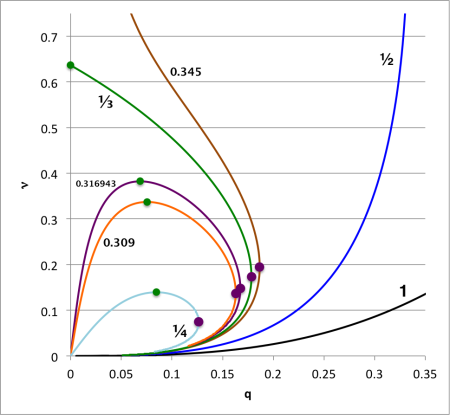
Following HC41 and SC42, we have found it particularly useful to label each equilibrium model according to the key structural parameters, and . The curves shown here on the right in Figure 2 graphically present the relationship for bipolytropic model sequences that have a variety of molecular-weight jumps, , at the core-envelope interface, as labeled. Along each Fig. 2 sequence for which , the green filled circle identifies the model with the largest mass ratio, . This maximum-mass model is a polytropic analogue of the Schönberg-Chandrasekhar mass limit, which was identified by HC41 and SC42 in the context of their studies of stars with isothermal cores.
- The maximum-mass model's position along each sequence has been determined analytically by setting
-
By solving the LAWE associated with various models along each equilibrium sequence, we have shown that the eigenfrequency of the fundamental-mode of radial oscillation is zero for each one of these maximum-mass models.
- Solutions to the LAWE were initially obtained via numerical integration techniques, in which case we were only able to make this association approximately;
- To our surprise, we also have been able to determine analytically an expression that defines the eigenfunction of the marginally unstable equilibrium model along each sequence ; as a result we have been able to show that the eigenfrequency associated with the maximum-mass model is precisely zero.
indexes, as labeled, over the range .
|
Figure 2: Equilibrium Sequences of Bipolytropes with and Various |
Analytically Determined Parameters† |
|||
|
|
|
|
|
|
|
|
0.0 | |||
|
0.33 |
24.00496 | 0.038378833 | 0.52024552 | |
|
0.316943 |
10.744571 | 0.068652714 | 0.382383875 | |
|
0.31 |
9.014959766 | 0.0755022550 | 0.3372170064 | |
|
0.3090 |
8.8301772 | 0.076265588 | 0.331475715 | |
|
|
4.9379256 | 0.084824137 | 0.139370157 | |
|
†Additional model parameters can be found here. |
||||
|
In terms of mass , length , and time , the units of various physical constants and variables are:
As a result, for example (see details below), if we hold the central-density — as well as and — constant along an equilibrium sequence, mass will scale as …
If instead (see details below) we hold — as well as and — constant along an equilibrium sequence, mass will scale as …
|
Original Model Construction[edit]
Fixed Central Density[edit]
From Examples, we find,
|
|
|
|
|
|
|
|
|
|
|
|
|
|
|
|
where, rewriting the relevant expressions in terms of the parameters,
and
we find,
|
|
|
|
|
|
|
|
|
|
|
|
|
|
|
|
|
|
|
|
|
|
|
|
|
|
|
|
|
|
|
|
Fixed Interface Pressure[edit]
Equilibrium Sequence Expressions[edit]
From the relevant interface conditions, we find,
|
|
|
|
Inverting this last expression gives,
|
|
|
|
|
|
|
|
Hence, keeping and constant, we have,
|
|
|
|
|
|
|
|
|
|
|
|
|
|
|
|
|
|
|
|
|
|
|
|
|
|
|
|
|
|
|
|
|
|
|
|
This last expression shows that if and are both held fixed, then the interface pressure, , will be constant along the sequence of equilibrium models.
Note also:
|
|
|
|
|
|
|
|
|
|
|
|
|
|
|
|
Fixed Interface Pressure Sequence Plots[edit]
A plot of versus at fixed interface pressure will be generated via the relations,
| Ordinate: | Abscissa: | |
|
|
vs |
|
Alternatively, a plot of versus at fixed interface pressure will be generated via the relations,
| Ordinate: | Abscissa: | |
|
|
vs |
|
|
The expression for is …
The extremum in occurs when the LHS of this expression is zero, that is, when …
For the solution to this expression is . |
|
|
|
Equilibrium Sequences of BiPolytropes Having |
||
| (Interface Pressure vs. Radius (Fixed Total Mass) |
Mass vs. Radius (Fixed Interface Pressure) |
Mass vs. Central Density (Fixed Interface Pressure) |
 |
|
|
|
|
|
|
| NOTE: In all three diagrams, the dashed vertical line identifies the value of the abscissa when it is evaluated for the interface location, . In each case, this vertical line intersects a key turning point along the model sequence. | ||


| |||||||||||||||||||||
Temporary Excel Interpolations[edit]
HERE
| Properties of Turning-Points Along Sequences Having Various | |||||
| (Fixed ) | (Fixed ) | ||||
| 1.000 | 1.6684629814 | 12.03999149 | 0.092175036 | 3.46986909 | 0.712724159 |
| 0.9 | 1.4459132276 | 13.67957562 | 0.091291571 | 3.50879154 | 0.688526899 |
| 0.8 | 1.0482530437 | 17.09391244 | 0.086279818 | 3.69798999 | 0.58112284 |
| 0.75 | 0.7170001608 | 20.48027265 | 0.079651055 | 3.91920968 | 0.484075667 |
| 0.74 | 0.6365283705 | 21.40307774 | 0.0777495 | 3.97973335 | 0.464464039 |
Fixed Total Mass[edit]
Equilibrium Sequence Expressions[edit]
Again, drawing from previous Examples in which — as well as and — is held fixed, equilibrium models obey the relations,
|
|
|
|
|
|
|
|
|
|
|
|
Let's invert the first expression in order to construct equilibrium sequences in which the total mass — rather than — is held fixed. We find that,
|
|
|
|
|
|
|
|
|
|
|
|
|
|
|
|
And,
|
|
|
|
|
|
|
|
|
|
|
|
Note as well that,
|
|
|
|
|
|
|
|
|
|
|
|
Sequence Plots[edit]
A plot of versus at fixed total mass will be generated via the relations,
| Ordinate | Abscissa | |
|
|
vs |
|

Hidden Text[edit]
Following the Lead of Yabushita75[edit]
Here in the context of bipolytropes, we want to construct an interface-pressure versus volume plot; and mass-versus-central density plots like the ones displayed for truncated isothermal spheres in Figure 1 of an accompanying discussion, and as displayed for a bipolytrope in Figure 1 (p. 445) of 📚 S. Yabushita (1975, MNRAS, Vol. 172, pp. 441 - 453).
In our accompanying chapter that presents example models of bipolytropes, we have adopted the following normalizations:
|
|
|
|
; |
|
|
|
|
|
|
|
; |
|
|
|
Also, from the relevant interface conditions, we find,
|
|
|
|
Inverting this last expression gives,
|
|
|
|
|
|
|
|
Hence, we can rewrite the "normalized" expressions as follows:
|
|
|
|
|
|
|
|
|
|
|
|
|
|
|
|
Fixed Interface Pressure[edit]
Start with the model relation,
|
|
|
|
|
|
|
|
Now, given that,
|
|
|
|
|
|
|
|
Fixed Total Mass[edit]
Also, from the relevant interface conditions, we find,
|
|
|
|
Inverting this last expression gives,
|
|
|
|
|
|
|
|
Hence, for a given specification of the interface location, — test values shown (in parentheses) assuming and — the desired expression for the central density is,
|
|
|
|
and, drawing the expression for the normalized total mass from our accompanying table of parameter values, namely,
|
|
|
|
we find,
|
|
|
|
|
|
|
|
|
|
|
|
|
|
|
|
|
|
|
|
where — again, from our accompanying table of parameter values —
|
|
|
|
(0.96077) | |
|
|
|
|
(0.79941) | |
|
|
|
|
(0.96225) | |
|
|
|
|
(1.10940) | |
|
|
|
|
(3.13637) | |
|
|
|
|
(2.77623) | |
|
|
|
|
(1.22153) |
Building on Earlier Eigenfunction Details[edit]
In the heading of Figure 6 from our accompanying presentation of the properties of marginally unstable oscillation modes in bipolytropes, we point to the (Excel spreadsheet) "Data File" that contains most of the relevant model details. See specifically,
|
in Marginally Unstable Models having Various |
|---|
Relevant Instabilities[edit]
Abstract[edit]
The analysis presented by 📚 Eggleton, Faulkner, & Cannon (1998) is essentially an analysis of the diagram. We can determine analytically at what value of the core-to-total mass ratio reaches a maximum () for various values of . For example, . Our LAWE analysis shows that none of these turning points is associated with the onset of a dynamical instability.
On the other hand, our LAWE analysis does identify a marginally unstable equilibrium configuration along every sequence; even sequences with . For example, .
Truncated n = 5 Polytrope[edit]
In Figure 3 of an accompanying discussion, we show where various turning points lie along the equilibrium sequence of truncated polytropes.
|
Figure 3: Equilibrium Sequences of Pressure-Truncated, n = 5 Polytropic Spheres |
|||||
| ● | †External Pressure vs. Volume (Fixed Mass) |
Mass vs. Radius (Fixed External Pressure) |
‡Mass vs. Central Density (Fixed External Pressure) |
Mass vs. Central Density (Fixed Radius) |
|
| ● | √3 | (a) |
(b) |
(c) |
(d) |
| ● | 3 | ||||
| ● | √15 | ||||
| ● | 9.01 | ||||
vs.
|
vs. |
vs. |
vs. |
||
-
KEY RESULT:
- The maximum "Bonnor-Ebert type" mass and external pressure occurs along the sequence precisely at .
- It is precisely at this turning point that the equilibrium model is marginally (dynamically) unstable; the eigenfunction is parabolic.
- For all , the location along the relevant sequence presents an analogous turning point whose location and whose eigenfunction is known analytically.
Bipolytropes with (nc, ne) = (5, 1)[edit]
q - ν Sequence Plots[edit]
In Figure 1 of an accompanying discussion, we show — via a plot in the diagram — how the bipolytrope sequence behaves for various values of the molecular-weight ratio over the range, .
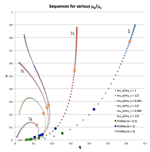
Figure 1: Analytically determined plot of fractional core mass () versus fractional core radius () for bipolytrope model sequences having six different values of : 1 (blue diamonds), ½ (red squares), 0.345 (dark purple crosses), ⅓ (pink triangles), 0.309 (light green dashes), and ¼ (purple asterisks). Along each of the model sequences, points marked by solid-colored circles correspond to models whose interface parameter, , has one of three values: 0.5 (green circles), 1 (dark blue circles), or 3 (orange circles); the images linked to Table 2 provide plots of the density, pressure and mass profiles for nine of these identified models.
According to our accompanying discussion, in terms of the parameters,
and
the parameter, , varies with as,
KEY RESULT: Over the range, , there is a value of above which no equilibrium configurations exist. We have determined the location of this "turning point" by setting, ; our derived result is,
Maximum Fractional Core Mass, (solid green circular markers)
for Equilibrium Sequences having Various Values ofLHS
RHS
--- --- --- --- --- --- --- 0.0 0.33
24.00496 0.0719668 0.0710624 0.2128753 0.0726547 1.8516032 -223.8157 -223.8159 0.038378833 0.52024552 0.316943
10.744571 0.1591479 0.1493938 0.4903393 0.1663869 2.1760793 -31.55254 -31.55254 0.068652714 0.382383875 0.3090
8.8301772 0.1924833 0.1750954 0.6130669 0.2053811 2.2958639 -18.47809 -18.47808 0.076265588 0.331475715 4.9379256 0.3309933 0.2342522 1.4179907 0.4064595 2.761622 -2.601255 -2.601257 0.084824137 0.139370157 Recall that,
and
The EFC98 Sequence Plot[edit]
📚 Eggleton, Faulkner, & Cannon (1998) also analytically determined the structure of models along various sequences; their Figure 1 displays the behavior of vs. for a range of . Note that,
KEY RESULT (to be done): From our original derivation, we have generated a plot intended to replicate Figure 1 from EFC98; then we have marked on each sequence the location of the mass-extremum (i.e., when ) as determined by our above analytically derived result.
Yabushita75 Guidance[edit]
Alternatively, as derived above, setting leads to the expression,
For the solution to this expression is . For other parameter choices, see here, for example.
LAWE Sol'n Max. Mtot 1 1.6686460157 1.668462981 2.2792811317 n/a Related Discussions[edit]
- Instability Onset Overview
- Analytic

Appendices: | VisTrailsEquations | VisTrailsVariables | References | Ramblings | VisTrailsImages | myphys.lsu | ADS |
